Linear Regression
Definition
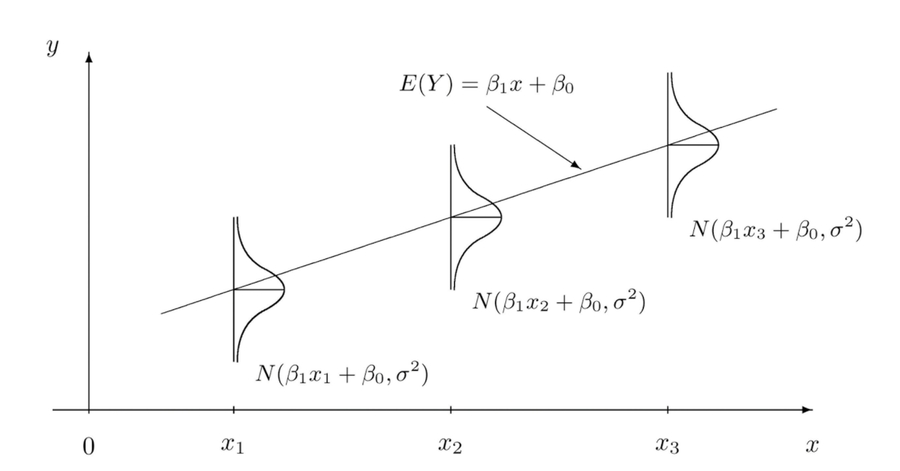
Linear regression is a linear model, which a linear relationship between the input and output . More technical, we can consider y y y can be a linear combination of X X X
Representation
Y = β 0 + β 1 X + ϵ Y= \beta_0+\beta_1X+\epsilon Y = β 0 + β 1 X + ϵ
How to determine this model?loss function?
最小二乘法least square推导loss function
L o s s = min β 0 , β 1 ∑ i = 1 n ( y i − β 0 + β 1 X i ) 2 Loss =\min_{\beta_0,\beta_1} \sum_{i=1}^{n}(y_i-\beta_0+\beta_1X_i)^2 L oss = min β 0 , β 1 ∑ i = 1 n ( y i − β 0 + β 1 X i ) 2
最大似然估计MLE(maximum likelihood estimation)推导loss function
what is mle?
用参数估计的方法,在有了一定的观测值之后,来找parameter,让我们可以最有可能看到我们观测值,让我们可以最大程度放大我们的观测值
estimating the parameters
finding the parameter values
maximize the likelihood(making the observation given the parameters)
推导过程(Y follws什么distribution?)
p ( Y i ∣ X i ) = 1 σ ( 2 π ) e − 1 2 σ 2 ( Y i − β ˉ 0 − β ˉ 1 X i ) 2 p(Y_i\vert X_i)=\frac{1}{\sigma(2\pi)}e^{-\frac{1}{2\sigma^2}(Y_i-\bar{\beta}_0-\bar{\beta}_1X_i)^2} p ( Y i ∣ X i ) = σ ( 2 π ) 1 e − 2 σ 2 1 ( Y i − β ˉ 0 − β ˉ 1 X i ) 2
L ( β ˉ 0 , β ˉ 1 , σ 2 ) = p ( Y 1 , ⋯ , Y n ∣ X 1 , ⋯ , X n ) = 1 σ n ( 2 π ) n / 2 e − 1 2 σ 2 ∑ i = 1 n ( Y i − β ˉ 0 − β ˉ 1 X i ) 2 L(\bar{\beta}_0,\bar{\beta}_1,\sigma^2)=p(Y_1,\cdots,Y_n\vert X_1,\cdots,X_n)=\frac{1}{\sigma^{n}(2\pi)^{n/2}}e^{-\frac{1}{2\sigma^2}\sum_{i=1}^n(Y_i-\bar{\beta}_0-\bar{\beta}_1X_i)^2} L ( β ˉ 0 , β ˉ 1 , σ 2 ) = p ( Y 1 , ⋯ , Y n ∣ X 1 , ⋯ , X n ) = σ n ( 2 π ) n /2 1 e − 2 σ 2 1 ∑ i = 1 n ( Y i − β ˉ 0 − β ˉ 1 X i ) 2
两者的关系
当他们在linear regression下的assumption下,这两个方法得到结果是相通的
one is from statistics, and the other one is from optimization
一些提醒
noise是数据造成的,是inherent bias. error是模型造成的,是人为的。是两个不同的概念
我们只能系统的保证其不会偏差(E ( Y ) = μ E(Y)=\mu E ( Y ) = μ )
null hypothesis : β 1 = 0 \beta_1=0 β 1 = 0
目的是从统计上来判断这组数据和population相差多少,assessing the accuracy of the coefficient estimation,可以使用 ppp-value 或者是 confidence interval
选择的统计量t = β ^ 1 − 0 S E ( β ^ 1 ) t=\frac{\hat{\beta}_1-0}{SE(\hat{\beta}_1)} t = SE ( β ^ 1 ) β ^ 1 − 0 distribution with n − 2 n-2 n − 2 degrees of freedom assuming β 1 = 0 \beta_1=0 β 1 = 0
How can we compare this model with others model?
(这个相当于模型外的判断模型的好坏 i.e. the extent to which the model fits the data)
assessing the overall accuracy
R S E = 1 n − 2 R S S = 1 n − 2 ∑ i n ( y i − y ^ i ) 2 RSE=\sqrt{\frac{1}{n-2}RSS}=\sqrt{\frac{1}{n-2}\sum_i^{n}(y_i-\hat{y}_i)^2} RSE = n − 2 1 RSS = n − 2 1 ∑ i n ( y i − y ^ i ) 2
R 2 = T S S − R R R T S S = 1 − R S S ∑ i n ( y i − y ^ i ) 2 R^2=\frac{TSS-RRR}{TSS}=1-\frac{RSS}{\sum_i^{n}(y_i-\hat{y}_i)^2} R 2 = TSS TSS − RRR = 1 − ∑ i n ( y i − y ^ i ) 2 RSS
where TSSTSSTSS is total sum of squares, RSSRSSRSS is the residual sum of squares(对误差的多少)
当是simple regression时,他相同于correlation
这里相当于 proportion of variability in that can be explained using ( 的变化中能够被解释的部分的比例 )
Multilinear Regression
Logistic Regression
图形/值域的理解
采用这个方法:x → p ( x ) → y x \rightarrow p(x) \rightarrow y x → p ( x ) → y
首先用 x x x 去拟合 概率p ( x ) p(x) p ( x )
然后用p p p 再去拟合y y y (采用threshold)
p ( x ) = e f ( x ) 1 + e f ( x ) = 1 1 + e − f ( x ) p(x)=\frac{e^{f(x)}}{1+e^{f(x)}}=\frac{1}{1+e^{-f(x)}} p ( x ) = 1 + e f ( x ) e f ( x ) = 1 + e − f ( x ) 1
Y Y Y 是得病不得病,p p p 是相当于肿瘤的指数, X X X 是关于肿瘤的input(size,位置,etc)
p ( Y = y i ) = p y i ( 1 − p ) 1 − y i , 0 < p < 1 , y i = 0 , 1 p(Y=y_i)=p^{y_i}(1-p)^{1-y_i},\ 0<p<1,\ y_i=0,1 p ( Y = y i ) = p y i ( 1 − p ) 1 − y i , 0 < p < 1 , y i = 0 , 1
l o g p ( X ) 1 − p ( X ) = β 0 + β 1 X log\frac{p(X)}{1-p(X)} = \beta_0+\beta_1X l o g 1 − p ( X ) p ( X ) = β 0 + β 1 X
How to determine this model?loss function?
Using MLE to get the loss function(面试必考题)
Key:Y fellows 什么distribution?
P ( Y = y i ∣ X ) = p y i ( 1 − p ) 1 − y i , 0 < p < 1 , y i = 0 , 1 P(Y=y_i\vert X) = p^{y_i}(1-p)^{1-y_i}, \ 0<p<1,\ y_i=0,1 P ( Y = y i ∣ X ) = p y i ( 1 − p ) 1 − y i , 0 < p < 1 , y i = 0 , 1
p = h β ( x i ) = 1 1 + e − β 0 + β 1 x p=h_{\beta}(x_i)=\frac{1}{1+e^{-\beta_0+\beta_1x}} p = h β ( x i ) = 1 + e − β 0 + β 1 x 1
L ( β ^ 0 , β ^ 1 ) = Π i = 1 n P ( Y i ∣ X i ) = Π i = 0 n p y i ( 1 − p ) 1 − y i = Π i = 0 n h β ( x i ) y i ( 1 − h β ( x i ) ) 1 − y i L(\hat\beta_0,\hat \beta_1)=\Pi_{i=1}^{n}P(Y_i \vert X_i)= \Pi_{i=0}^n p^{y_i}(1-p)^{1-y_i}=\Pi_{i=0}^n {h_{\beta}(x_i)}^{y_i}(1-h_{\beta}(x_i))^{1-y_i} L ( β ^ 0 , β ^ 1 ) = Π i = 1 n P ( Y i ∣ X i ) = Π i = 0 n p y i ( 1 − p ) 1 − y i = Π i = 0 n h β ( x i ) y i ( 1 − h β ( x i ) ) 1 − y i
如何调参呢?有没有类似与linear的t distribution之类的?
t distribution?something?
How can we compare this model with others model?
link: Confusion matrix/AUC
Compare with linear regression
Step1: ‘Given ,得的distribution’——这是机器学习模型利用数据可以解决的问题
Step2: ‘根据的distribution,得到的取值’——判断怎么用是你的问题
Multiple Logistic Regression
p ( x ) = h β ( x i ) = 1 1 + e g ( x ) , where g ( x ) = β 0 + β 1 , 1 x 1 + β 1 , 2 x 1 2 + β 2 x 2 p(x)=h_{\beta}(x_i)=\frac{1}{1+e^{g(x)}}, \ \textit{where }\ g(x)=\beta_0+\beta_{1,1}x_1+\beta_{1,2}x_1^2+\beta_2x_2 p ( x ) = h β ( x i ) = 1 + e g ( x ) 1 , where g ( x ) = β 0 + β 1 , 1 x 1 + β 1 , 2 x 1 2 + β 2 x 2
你会面对一个(overfit/underfit)的问题:
模型复杂提到,可以更好的对应training data,但是对testing data不一定好
过度拟合就是overfitting,但是过少可能就underfitting
很多时候,多分类问题可以比较成为多个两分类问题,两两二分类来做
Regularization——Ridge regression/Lasso regression
SVM
E ( ( w T x + b , 0 ) max ) E((w^Tx+b,0)_{\max}) E (( w T x + b , 0 ) m a x )
Maximum margin classifier max 1 ∣ ∣ w ∣ ∣ , s . t . y i ( w T x i + b ) ≥ 0 , i = 1 , ⋯ \max \frac{1}{\vert \vert w \vert \vert},\qquad s.t. y_i(w^Tx_i+b)\geq 0,\qquad i=1,\cdots max ∣∣ w ∣∣ 1 , s . t . y i ( w T x i + b ) ≥ 0 , i = 1 , ⋯
min 1 2 ∣ ∣ w ∣ ∣ 2 , s . t . y i ( w T x i + b ) ≥ 1 , i = 1 , ⋯ , n \min \frac{1}{2}\vert\vert w \vert\vert^2,\qquad s.t. y_i(w^Tx_i+b)\geq 1,\qquad i=1,\cdots,n min 2 1 ∣∣ w ∣ ∣ 2 , s . t . y i ( w T x i + b ) ≥ 1 , i = 1 , ⋯ , n
dual L ( w , b , a ) = 1 2 ∣ ∣ w ∣ ∣ 2 − ∑ i = 1 n α i ( y i ( w T x i + b ) − 1 ) \mathcal{L}(w,b,a)=\frac{1}{2}\vert \vert w\vert \vert^2-\sum_{i=1}^n \alpha_i(y_i(w^Tx_i+b)-1) L ( w , b , a ) = 2 1 ∣∣ w ∣ ∣ 2 − ∑ i = 1 n α i ( y i ( w T x i + b ) − 1 )
L ( w , b , a ) = ∑ i = 1 n α i − 1 2 α i α j y i y j x i T x j \mathcal{L}(w,b,a)=\sum_{i=1}^n\alpha_i-\frac{1}{2}\alpha_i\alpha_jy_i y_jx_i^T x_j L ( w , b , a ) = ∑ i = 1 n α i − 2 1 α i α j y i y j x i T x j and w = ∑ i = 1 n α i y i x i w=\sum_{i=1}^n\alpha_iy_ix_i w = ∑ i = 1 n α i y i x i
换成核估计
f ( x ) = ∑ i = 1 N w i ϕ i ( x ) + b f(x)=\sum_{i=1}^Nw_i\phi_i(x)+b f ( x ) = ∑ i = 1 N w i ϕ i ( x ) + b 转换成为 f ( x ) = ∑ i = 1 l α i y i ⟨ ϕ ( x i ) , ϕ ( x ) ⟩ + b f(x)=\sum_{i=1}^l\alpha_i y_i \langle \phi(x_i), \phi(x) \rangle+b f ( x ) = ∑ i = 1 l α i y i ⟨ ϕ ( x i ) , ϕ ( x )⟩ + b
α \alpha α 可以由dual 来求
max α ∑ i = 1 n α i − 1 2 ∑ i , j = 1 n α i α j y i y j ⟨ ϕ ( x i ) ϕ ( x j ) ⟩ s . t . α i ≥ 0 , i = 1 , ⋯ , n ; ∑ i = 1 n α i y i = 0 \max_{\alpha}\sum_{i=1}^n \alpha_i-\frac{1}{2}\sum_{i,j=1}^n\alpha_i\alpha_jy_iy_j\langle \phi(x_i)\phi(x_j)\rangle \qquad s.t. \alpha_i \geq 0,i=1,\cdots, n; \sum_{i=1}^n\alpha_iy_i=0 max α ∑ i = 1 n α i − 2 1 ∑ i , j = 1 n α i α j y i y j ⟨ ϕ ( x i ) ϕ ( x j )⟩ s . t . α i ≥ 0 , i = 1 , ⋯ , n ; ∑ i = 1 n α i y i = 0
max α ∑ i = 1 n α i − 1 2 ∑ i , j = 1 n α i α j y i y j x i x j s . t . α i ≥ 0 , i = 1 , ⋯ , n ; ∑ i = 1 n α i y i = 0 \max_{\alpha}\sum_{i=1}^n \alpha_i-\frac{1}{2}\sum_{i,j=1}^n\alpha_i\alpha_jy_iy_jx_ix_j \qquad s.t. \alpha_i \geq 0,i=1,\cdots, n; \sum_{i=1}^n\alpha_iy_i=0 max α ∑ i = 1 n α i − 2 1 ∑ i , j = 1 n α i α j y i y j x i x j s . t . α i ≥ 0 , i = 1 , ⋯ , n ; ∑ i = 1 n α i y i = 0
Last updated 11 months ago